vnorm
vnorm
![]()

vnorm provides tools for sampling, visualizing, and projecting near
real algebraic varieties defined by polynomial equations. It implements
the variety normal distribution using mpoly for polynomial
representations and Stan-based samplers. In addition to sampling with
rvnorm(), the package includes pseudo-density evaluation via
pdvnorm(), ggplot2 visualization with geom_variety(), and projection
onto varieties with project_onto_variety().
Installation
You can install the development version of vnorm from GitHub with:
if (!requireNamespace("devtools")) install.packages("devtools")
devtools::install_github("dkahle/mpoly")
devtools::install_github("sonish13/vnorm")
rvnorm() uses Stan/HMC as the primary sampling backend, so you should
install cmdstanr and CmdStan for normal package use. A rejection
sampler interface is also available (rejection = TRUE) and can be
useful for quick examples or simple low-dimensional cases.
Quick Start: Sample and Plot a Variety
The main workflow is: define a polynomial variety, sample near it with
rvnorm(), and visualize with geom_variety().
Stan/HMC (primary path):
p1 <- mp("x^2 + y^2 - 1")
samps1 <- rvnorm(
  2000,
  poly = p1,
  sd = 0.1,
  output = "tibble"
)

ggplot(samps1, aes(x, y)) +
  geom_point(size = 0.4) +
  geom_variety(poly = p1, inherit.aes = FALSE, show.legend = FALSE) +
  coord_equal() +
  theme_minimal()
Main Functions
rvnorm()samples from a variety normal distribution near a polynomial variety.pdvnorm()evaluates the pseudo-density (up to a normalizing constant).geom_variety()plots real 1D varieties in 2D usingggplot2.project_onto_variety()projects points onto a variety.compile_stan_code()pre-compiles reusable Stan models for repeated sampling with related polynomial forms.
rvnorm(): the main sampling function
rvnorm() is the main entry point for sampling near varieties defined
by one polynomial (mpoly) or a system of polynomials (mpolyList). It
supports:
- Stan/HMC sampling (default; best for most serious use)
- rejection sampling (
rejection = TRUE; good for quick examples and simple cases) - built-in pre-compiled Stan models (
pre_compiled = TRUE) for common polynomial structures - user pre-compiled Stan models (
user_compiled = TRUE) for repeated sampling of related polynomial forms
Common arguments:
poly: the polynomial or polynomial system defining the target varietysd/Sigma: controls concentration around the varietyoutput: output format (for example"tibble")w: window size for unbounded varieties (and for rejection sampling)rejection: use the rejection sampler instead of Stan/HMC
The Stan/HMC path is the default and recommended mode for most use. The rejection sampler is available as a lighter-weight alternative for some low dimensional examples.
Default Stan/HMC usage:
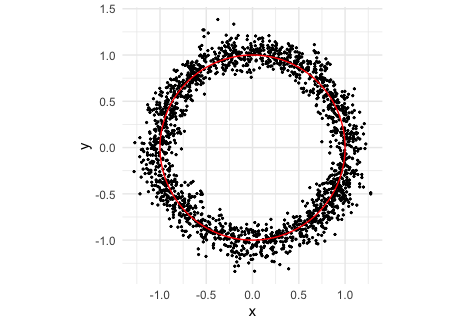
p2 <- mp("x^2 + y^2 - 1")
samps2 <- rvnorm(2000, poly = p2, sd = 0.1, output = "tibble")
Typical default workflow (sample, then visualize), shown above:
p2 <- mp("x^2 + y^2 - 1")
samps2 <- rvnorm(2000, poly = p2, sd = 0.1, output = "tibble")

ggplot(samps2, aes(x, y)) +
  geom_point(size = 0.5, alpha = 0.35) +
  geom_variety(poly = p2, inherit.aes = FALSE) +
  coord_equal()
Additional common rvnorm() usage patterns:
# Use a packaged pre-compiled Stan model when available (small degree/variable cases)
rvnorm(2000, mp("x^2 + y^2 + z^2 - 1"), sd = 0.1, pre_compiled = TRUE)

# Unbounded varieties typically need a window parameter w
rvnorm(2000, mp("x y - 1"), sd = 0.1, w = 2, output = "tibble")

# Multi-polynomial systems (underdetermined / overdetermined are both supported)
rvnorm(2000, mp(c("x^2 + y^2 + z^2 - 1", "z")), sd = 0.1, output = "tibble")

# Use Sigma for anisotropic concentration (single polynomial)
rvnorm(2000, mp("x^2 + y^2 - 1"), Sigma = diag(c(0.02, 0.10)^2), output = "tibble")

# Use Sigma with polynomial systems as well
rvnorm(2000, mp(c("x^2 + y^2 - 1", "x y - 0.25")), Sigma = diag(c(0.05, 0.08)^2))
Rejection sampler usage (alternative path; currently the wrapper
supports scalar sd):
set.seed(1)
p3 <- mp(c("x^2 + y^2 - 1", "x y - 0.25"))
samps3 <- rvnorm(
  2000,
  poly = p3,
  sd = 0.1,
  rejection = TRUE,
  w = 1.5,
  output = "tibble"
)

ggplot(samps3, aes(x, y)) +
  geom_point(size = 0.5, alpha = 0.4) +
  geom_variety(poly = p3, xlim = c(-2, 2), ylim = c(-2, 2), inherit.aes = FALSE) +
  coord_equal() +
  theme_minimal()
pdvnorm(): pseudo-density evaluation
pdvnorm() can be used with single polynomials and polynomial systems,
and supports scalar, vector, or matrix sigma inputs depending on the
setting.
p4 <- mp(c("x^2 + y^2 - 1", "x y - 0.25"))
x1 <- c(0.8, 0.3)

pdvnorm(x1, p4, sigma = 1)
#> [1] 0.1560083
pdvnorm(x1, p4, sigma = c(1, 2), homo = FALSE)
#> [1] 0.1085086
pdvnorm(x1, p4, sigma = diag(c(1, 4)))
#> [1] 0.07810636
geom_variety(): ggplot2-compatible variety plots
geom_variety() supports both single-polynomial (mpoly) and
multi-polynomial (mpolyList) inputs and works with standard ggplot2
themes/scales. It now defaults to a 201 x 201 contouring grid and
projection = "auto", which projects extracted contours back onto
poly = 0 whenever a shift is used, when the plotting grid has no
strict sign change, or when the raw contour drifts noticeably off the
zero set. Use projection = "off" to inspect the raw shifted level set
directly, or projection = "on" to always project.
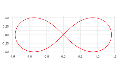
p5 <- mp("(x^2 + y^2)^2 - 2 (x^2 - y^2)")

ggplot() +
  geom_variety(poly = p5, xlim = c(-2, 2), ylim = c(-2, 2), show.legend = FALSE) +
  coord_equal() +
  theme_minimal()
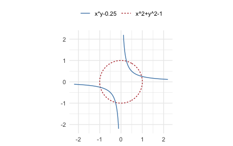
p6 <- mp(c("x^2 + y^2 - 1", "x y - 0.25"))

ggplot() +
  geom_variety(
    poly = p6,
    xlim = c(-2, 2),
    ylim = c(-2, 2),
    vary_colour = TRUE
  ) +
  coord_equal() +
  scale_colour_manual(values = c("steelblue", "firebrick")) +
  theme_minimal() +
  theme(legend.position = "top")
If a squared polynomial (for example, p^2) produces no contour at
shift = 0, geom_variety() prints a suggested negative shift. Using
that shift can help recover the plotted zero set in no-sign-change
cases. With the default projection = "auto", the shifted contour is
then projected back onto the actual zero set; this usually improves
repeated-factor plots, although hard singular cases can still miss
branches.
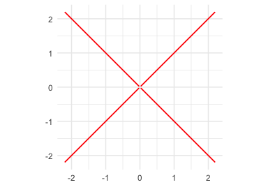
p7 <- mp("y^2 - x^2")
ggplot() +
  geom_variety(poly = p7^2, xlim = c(-2, 2), ylim = c(-2, 2)) +
  coord_equal()
#> All values are positive on the plotting grid; try shift = -0.000562449.
#> Zero contours were generated
p7 <- mp("y^2 - x^2")
ggplot() +
  geom_variety(
    poly = p7^2,
    xlim = c(-2, 2), ylim = c(-2, 2),
    shift = -0.000959513,
    show.legend = FALSE
  ) +
  coord_equal() +
  theme_minimal()
#> Using shift = -0.000959513 to contour a nearby level set. For repeated-factor varieties, the projected result may still miss branches; if the unsquared polynomial is available, prefer plotting that directly.
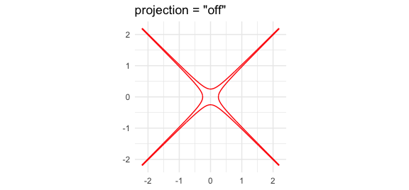
p7_cross <- mp("y^2 - x^2")
ggplot() +
geom_variety(
poly = p7_cross^2,
xlim = c(-2, 2), ylim = c(-2, 2),
shift = -0.004,
projection = "off",
show.legend = FALSE
) +
coord_equal() +
ggtitle('projection = "off"') +
theme_minimal()
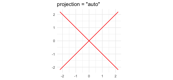
ggplot() +
geom_variety(
poly = p7_cross^2,
xlim = c(-2, 2), ylim = c(-2, 2),
shift = -0.004,
projection = "auto",
show.legend = FALSE
) +
coord_equal() +
ggtitle('projection = "auto"') +
theme_minimal()
project_onto_variety(): projection with visualization
The projection functions are useful for snapping points back to a variety and for inspecting projection behavior visually.
p8 <- mp("x^2 + y^2 - 0.25")
x0 <- c(1.3, 0.9)
(x0_proj <- project_onto_variety(x0, p8))
#> [1] 0.4110961 0.2846050
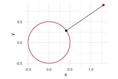
The red point is the starting value and the black point is its projection onto the variety. The grey segment shows the displacement from the starting point to the projected point.
Adaptive time stepping is used by default. The comparison below illustrates the homotopy projection path from the same starting point using fixed step sizes versus adaptive step sizes (similar to the paper figure). The open circles mark successive iterates along the path.
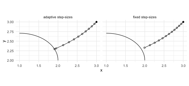
In each panel, the black curve is the target variety (an ellipse segment), the connected black path is the homotopy projection path from the same starting point, and the open circles show the successive iterates. The adaptive method is the default because it typically reaches the variety in fewer steps while maintaining the error tolerance.
Pre-compiled Models
vnorm includes pre-compiled Stan models for common polynomial
structures (up to three variables and total degree at most three). For
repeated work with a custom polynomial form, use compile_stan_code()
once and then call rvnorm() with user_compiled = TRUE on related
polynomials with different coefficients.
p_template <- mp("x^4 + y^4 - 1")
compile_stan_code(poly = p_template)

p_new <- mp("2 x^4 + 3 y^4 - 1")
samps_new <- rvnorm(1000, poly = p_new, sd = 0.1, user_compiled = TRUE)
Learn More
The README focuses on the main user-facing workflow: sample, visualize, evaluate, and project. A longer manuscript with the mathematical background and additional examples is in preparation and will be shared separately.
References
- Kahle, David and Hauenstein, Jonathan D. (2024). Stochastic Exploration of Real Varieties via Variety Distributions. arXiv:2410.16071
- Griffin, Zachary A. and Hauenstein, Jonathan D. (2015). Real solutions to systems of polynomial equations and parameter continuation. Advances in Geometry, 15(2), 173–187. doi:10.1515/advgeom-2015-0004